A tutorial to run diffdriver
diffdriver_tutorial.RmdEnvironmental requirement
Need 16G memory to run diffdriver. The place that needs the most memory is the parameter estimation for background mutation rate model.
Use an optimized BLAS library (important for speed)
The most time-consuming step in diffdriver is the parameter estimation for the background mutation rate model, which is dominated by dense matrix operations (the topic-model fit and the BFGS likelihood optimization). The speed of these operations depends almost entirely on the BLAS (Basic Linear Algebra Subprograms) library that R is linked against.
By default, R ships with an unoptimized reference BLAS, which can make the background mutation rate estimation many times slower (in our tests, a single run went from roughly 15 minutes with an optimized BLAS to over 90 minutes with the reference BLAS). We strongly recommend linking R against an optimized BLAS before running diffdriver:
-
macOS: use Apple’s Accelerate / vecLib BLAS, which is bundled with the R framework build. Point the BLAS symlink to the vecLib version (run once, in a shell):
To revert to the reference BLAS:
ln -sf libRblas.0.dylib libRblas.dylib. Note that reinstalling or updating R resets this symlink, so you may need to re-apply it. Linux: install and select an optimized BLAS such as OpenBLAS, e.g. on Debian/Ubuntu
sudo apt-get install libopenblas-devthensudo update-alternatives --config libblas.so.3(or build R against OpenBLAS / MKL).
You can check which BLAS R is currently using with
sessionInfo() or extSoftVersion()["BLAS"]. The
results in this tutorial were generated on the Dartmouth Discovery HPC
cluster, with the following configuration:
R version:     R version 4.4.3 (2025-02-28)
Platform:      x86_64-pc-linux-gnu
Running under: Red Hat Enterprise Linux 8.10 (Ootpa)
BLAS:          /usr/lib64/libopenblasp-r0.3.15.so
LAPACK:        /usr/lib64/libopenblasp-r0.3.15.so
On this cluster R is linked against OpenBLAS (an optimized BLAS), which is why the background mutation rate estimation completes quickly.
Prepare input
Diffdriver requires three datasets from the user: phenotype or context of each individual tumor sample, somatic mutations identified from tumor samples and a list of driver gene names. Diffdriver will test the association between the phenotype/context with selection strength of each provided driver gene.
- Phenotype/Context
Diffdriver needs phenotype or context of each individual tumor sample. A data frame should provided, in this data frame the first column is sample ID with column name “SampleID”, the second column is phenotype or context with the phenotype or context name as column name (note no space or in tab in column names are allowed). See an example below:
phenof = system.file("extdata/", "example_phenotypes.txt", package = "diffdriver")
pheno <- read.table(phenof, header = T)
head(pheno)
#>                       SampleID SmokingCessation
#> 1 TCGA-N5-A4R8-01A-11D-A28R-08        0.5319630
#> 2 TCGA-N5-A4RD-01A-11D-A28R-08        0.0448991
#> 3 TCGA-N5-A4RF-01A-11D-A28R-08       -0.3140750
#> 4 TCGA-N5-A4RJ-01A-11D-A28R-08        0.4229920
#> 5 TCGA-N5-A4RM-01A-11D-A28R-08       -0.2830070
#> 6 TCGA-N5-A4RN-01A-12D-A28R-08 0.7874080- Driver genes
A vector of driver gene names. Diffdriver will test the association for each gene.
genef = system.file("extdata", "example_gene.txt", package = "diffdriver")
gene <- read.table(genef, header = F)
head(gene)
#>       V1
#> 1   CHD4
#> 2 PIK3CA- Somatic mutations
Diffdriver needs the somatic mutations identified for each tumor samples. Note this should include all somatic mutations identified, not just the ones in selected driver genes. Somatic mutations will be used to estimate background mutation rate and selection strength for selected genes. A data frame should be provided, see below for colnames of this data frame and example mutations.
mutf = system.file("extdata/", "example_mutations.txt", package = "diffdriver")
mut <- read.table(mutf, header = T)
head(mut)
#>   Chromosome  Position Ref Alt                     SampleID
#> 1         19  55653236   C   T TCGA-N6-A4VE-01A-11D-A28R-08
#> 2         17  65134211   C   T TCGA-NA-A4R1-01A-11D-A28R-08
#> 3         20  30354424   G   T TCGA-N8-A4PM-01A-11D-A28R-08
#> 4          6  18215312   G   C TCGA-N8-A4PO-01A-11D-A28R-08
#> 5          1 154186393   C   G TCGA-NA-A4R0-01A-11D-A28R-08
#> 6 10 23003128 C A TCGA-NF-A4X2-01A-11D-A28R-08- Covariates (optional)
Optionally, the user can provide sample-level covariates (e.g. age, sex) to adjust for when testing the phenotype association. Either a path to a delimited file or a data frame can be supplied. It must contain a “SampleID” column plus one or more covariate columns, which may be numeric (e.g. age) or categorical (e.g. sex); categorical columns are automatically expanded into dummy variables. Only samples with complete covariate information are kept, and these are intersected with the mutation and phenotype samples. See an example below:
covf = system.file("extdata/", "example_covariates.txt", package = "diffdriver")
covariates <- read.table(covf, header = T)
head(covariates)
#>                       SampleID Age Sex
#> 1 TCGA-N5-A4R8-01A-11D-A28R-08  76   F
#> 2 TCGA-N5-A4RD-01A-11D-A28R-08  40   F
#> 3 TCGA-N5-A4RF-01A-11D-A28R-08  64   M
#> 4 TCGA-N5-A4RJ-01A-11D-A28R-08  49   F
#> 5 TCGA-N5-A4RM-01A-11D-A28R-08  75   M
#> 6 TCGA-N5-A4RN-01A-12D-A28R-08  57   M
In addition to these datasets provided by the user, diffdriver also needs annotation files. See the package installation page for download links to these annotation files. Unless the number of tumor samples or number of mutations is very small, we suggest to use the 96-annotation files. Please download these files to a folder and provide the folder address to diffdriver.
- Directory that contains annotation files
annodir = "/Volumes/Szhao/library/diffdriver_anno/annodir96"
list.files(annodir)
#>  [1] "anno96_nttype1_annodata.txt"  "anno96_nttype10_annodata.txt"
#>  [3] "anno96_nttype11_annodata.txt" "anno96_nttype12_annodata.txt"
#>  [5] "anno96_nttype13_annodata.txt" "anno96_nttype14_annodata.txt"
#>  [7] "anno96_nttype15_annodata.txt" "anno96_nttype16_annodata.txt"
#>  [9] "anno96_nttype17_annodata.txt" "anno96_nttype18_annodata.txt"
#> [11] "anno96_nttype19_annodata.txt" "anno96_nttype2_annodata.txt"
#> [13] "anno96_nttype20_annodata.txt" "anno96_nttype21_annodata.txt"
#> [15] "anno96_nttype22_annodata.txt" "anno96_nttype23_annodata.txt"
#> [17] "anno96_nttype24_annodata.txt" "anno96_nttype25_annodata.txt"
#> [19] "anno96_nttype26_annodata.txt" "anno96_nttype27_annodata.txt"
#> [21] "anno96_nttype28_annodata.txt" "anno96_nttype29_annodata.txt"
#> [23] "anno96_nttype3_annodata.txt"  "anno96_nttype30_annodata.txt"
#> [25] "anno96_nttype31_annodata.txt" "anno96_nttype32_annodata.txt"
#> [27] "anno96_nttype33_annodata.txt" "anno96_nttype34_annodata.txt"
#> [29] "anno96_nttype35_annodata.txt" "anno96_nttype36_annodata.txt"
#> [31] "anno96_nttype37_annodata.txt" "anno96_nttype38_annodata.txt"
#> [33] "anno96_nttype39_annodata.txt" "anno96_nttype4_annodata.txt"
#> [35] "anno96_nttype40_annodata.txt" "anno96_nttype41_annodata.txt"
#> [37] "anno96_nttype42_annodata.txt" "anno96_nttype43_annodata.txt"
#> [39] "anno96_nttype44_annodata.txt" "anno96_nttype45_annodata.txt"
#> [41] "anno96_nttype46_annodata.txt" "anno96_nttype47_annodata.txt"
#> [43] "anno96_nttype48_annodata.txt" "anno96_nttype49_annodata.txt"
#> [45] "anno96_nttype5_annodata.txt"  "anno96_nttype50_annodata.txt"
#> [47] "anno96_nttype51_annodata.txt" "anno96_nttype52_annodata.txt"
#> [49] "anno96_nttype53_annodata.txt" "anno96_nttype54_annodata.txt"
#> [51] "anno96_nttype55_annodata.txt" "anno96_nttype56_annodata.txt"
#> [53] "anno96_nttype57_annodata.txt" "anno96_nttype58_annodata.txt"
#> [55] "anno96_nttype59_annodata.txt" "anno96_nttype6_annodata.txt"
#> [57] "anno96_nttype60_annodata.txt" "anno96_nttype61_annodata.txt"
#> [59] "anno96_nttype62_annodata.txt" "anno96_nttype63_annodata.txt"
#> [61] "anno96_nttype64_annodata.txt" "anno96_nttype65_annodata.txt"
#> [63] "anno96_nttype66_annodata.txt" "anno96_nttype67_annodata.txt"
#> [65] "anno96_nttype68_annodata.txt" "anno96_nttype69_annodata.txt"
#> [67] "anno96_nttype7_annodata.txt"  "anno96_nttype70_annodata.txt"
#> [69] "anno96_nttype71_annodata.txt" "anno96_nttype72_annodata.txt"
#> [71] "anno96_nttype73_annodata.txt" "anno96_nttype74_annodata.txt"
#> [73] "anno96_nttype75_annodata.txt" "anno96_nttype76_annodata.txt"
#> [75] "anno96_nttype77_annodata.txt" "anno96_nttype78_annodata.txt"
#> [77] "anno96_nttype79_annodata.txt" "anno96_nttype8_annodata.txt"
#> [79] "anno96_nttype80_annodata.txt" "anno96_nttype81_annodata.txt"
#> [81] "anno96_nttype82_annodata.txt" "anno96_nttype83_annodata.txt"
#> [83] "anno96_nttype84_annodata.txt" "anno96_nttype85_annodata.txt"
#> [85] "anno96_nttype86_annodata.txt" "anno96_nttype87_annodata.txt"
#> [87] "anno96_nttype88_annodata.txt" "anno96_nttype89_annodata.txt"
#> [89] "anno96_nttype9_annodata.txt"  "anno96_nttype90_annodata.txt"
#> [91] "anno96_nttype91_annodata.txt" "anno96_nttype92_annodata.txt"
#> [93] "anno96_nttype93_annodata.txt" "anno96_nttype94_annodata.txt"
#> [95] "anno96_nttype95_annodata.txt" "anno96_nttype96_annodata.txt"
Run diffdriver
To ensure that the numerical results are reproducible, this tutorial uses a fixed random seed.
With signature adjustment (BMRmode = "signature"), which
is the default mode, it will need around 15min to estimate parameters in
background model. Please use the provided the annotation folder with
96-annotation files when running with the “signature mode”.
res <- diffdriver(gene = gene, mut= mut, pheno = pheno, anno_dir = "/Volumes/Szhao/library/diffdriver_anno/annodir96", k=6, totalnttype = 96, BMRmode = "signature", output_dir = output_dir, output_prefix = "testdiffdriver_sig")
res
The result (re-using a previously computed run to avoid re-estimating the background model here):
             dd.p      mlr.p   mlr.v2.p  fisher.p  binom.p      lr.p    dd.fdr
CHD4   1.00000000 0.85864512 0.83477953 1.0000000 1.000000 0.7509494 1.0000000
PIK3CA 0.05397616 0.01370322 0.01300004 0.5576717 0.453489 0.1443223 0.1079523
          mlr.fdr mlr.v2.fdr fisher.fdr binom.fdr    lr.fdr mut.E1 mut.E0 E1 E0
CHD4   0.85864512 0.83477953          1 1.0000000 0.7509494      5      4 22 18
PIK3CA 0.02740643 0.02600007          1 0.9069781 0.2886446      7      9 22 18
Without signature adjustment (BMRmode = "regular"), it
will need around 15min to estimate parameters in background model. You
can use the provided the annotation folder with 9-annotation files or
96-annotation files. The example below uses 96-annotation files. When
total number of mutations is low, one should use 9-annotation files.
res <- diffdriver(gene = gene, mut= mut, pheno = pheno,  anno_dir = "/Volumes/Szhao/library/diffdriver_anno/annodir96", totalnttype = 96, BMRmode = "regular", output_dir = output_dir, output_prefix = "testdiffdriver_reg")
res
The result (re-using a previously computed run):
             dd.p      mlr.p   mlr.v2.p  fisher.p  binom.p      lr.p    dd.fdr
CHD4   1.00000000 0.85864512 0.83477953 1.0000000 1.000000 0.7509494 1.0000000
PIK3CA 0.03021595 0.01370322 0.01300004 0.5576717 0.453489 0.1443223 0.0604319
          mlr.fdr mlr.v2.fdr fisher.fdr binom.fdr    lr.fdr mut.E1 mut.E0 E1 E0
CHD4   0.85864512 0.83477953          1 1.0000000 0.7509494      5      4 22 18
PIK3CA 0.02740643 0.02600007          1 0.9069781 0.2886446      7      9 22 18
Adjusting for covariates
To adjust for sample-level covariates, pass them through the
covariates argument (a file path or a data frame). The
covariates are added to the model under both the null and alternative
hypotheses, so the phenotype effect for each gene is tested conditional
on the covariates. The example below adjusts for age and sex. It uses
the same parameters as the signature run above (k = 6,
BMRmode = "signature"); only the covariates
argument is new.
res_cov <- diffdriver(gene = gene, mut= mut, pheno = pheno, covariates = covariates, anno_dir = "/Volumes/Szhao/library/diffdriver_anno/annodir96", k=6, totalnttype = 96, BMRmode = "signature", output_dir = output_dir, output_prefix = "testdiffdriver_cov")
res_cov
The result (re-using a previously computed run). Adjusting for age
and sex strengthens the PIK3CA association relative to the signature run
above (dd.p 0.054 → 0.0045); CHD4 is unchanged:
              dd.p      mlr.p   mlr.v2.p  fisher.p  binom.p      lr.p     dd.fdr
CHD4   1.000000000 0.85864512 0.83477953 1.0000000 1.000000 0.7509494 1.00000000
PIK3CA 0.004509065 0.01370322 0.01300004 0.5576717 0.453489 0.1443223 0.00901813
          mlr.fdr mlr.v2.fdr fisher.fdr binom.fdr    lr.fdr mut.E1 mut.E0 E1 E0
CHD4   0.85864512 0.83477953          1 1.0000000 0.7509494      5      4 22 18
PIK3CA 0.02740643 0.02600007          1 0.9069781 0.2886446      7      9 22 18
Plot specific genes
To visualize the data for specific genes, diffdriver has a plotting function:
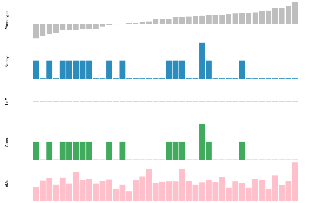
diffdriver::plot_mut(gene_name = "PIK3CA", mut= mut, pheno = pheno, totalnttype = 9, anno_dir = "/Volumes/Szhao/library/diffdriver_anno/annodir9")For PIK3CA, this produces the following plot. Each column is a tumor sample (ordered by phenotype); the rows show, from top to bottom, the phenotype, the number of nonsynonymous mutations, loss-of-function mutations, mutations at conserved sites, and the total mutation burden per sample:
Session information for the environment used to generate these results (Dartmouth Discovery HPC cluster):
R version 4.4.3 (2025-02-28)
Platform: x86_64-pc-linux-gnu
Running under: Red Hat Enterprise Linux 8.10 (Ootpa)

Matrix products: default
BLAS/LAPACK: /usr/lib64/libopenblasp-r0.3.15.so;  LAPACK version 3.9.0

attached base packages:
[1] stats     graphics  grDevices utils     datasets  methods   base

other attached packages:
[1] diffdriver_0.1.8

loaded via a namespace (and not attached):
[1] compiler_4.4.3    Matrix_1.7-5      grid_4.4.3        data.table_1.18.4
[5] lattice_0.22-9