Getting Started
2026-03-30
QuickStart.RmdWhat is scads?
scads (Single-Cell
ATAC-seq Disease
Scoring) computes per-cell disease relevance scores
from scATAC-seq data and GWAS summary statistics. Give it a peak-by-cell
count matrix and GWAS sumstats, and it returns a score for every cell
indicating how disease-relevant that cell’s chromatin profile is.
Runtime and resource requirements
| Step | What it does | Runtime (demo) | Peak memory |
|---|---|---|---|
| 1. fastTopics | Topic model fitting + DE testing | ~1 min | ~650 MB |
| 2. Annotations | Convert peaks to BED files | < 10 sec | Negligible |
| 3. S-LDSC | Stratified LD score regression per topic | ~8 min/topic (chr10 demo); ~1–2 hours/topic (all 22 chr) | ~300 MB/topic |
| 4. Cell scores | Combine enrichments with topic loadings | < 10 sec | ~650 MB |
Download S-LDSC reference data
scads requires reference files from the S-LDSC baseline
LD model. Download and extract them into a local directory (e.g.,
~/LDSCORE/). All files are available from Zenodo.
Disk usage: The compressed downloads total ~1 GB. After extraction, the reference data requires ~4 GB of disk space.
mkdir -p ~/LDSCORE && cd ~/LDSCORE

# Download reference files from Zenodo (~1 GB total)
curl -fSL -o 1000G_Phase3_plinkfiles.tgz \
  "https://zenodo.org/records/10515792/files/1000G_Phase3_plinkfiles.tgz?download=1"
curl -fSL -o 1000G_Phase3_baselineLD_v2.2_ldscores.tgz \
  "https://zenodo.org/records/10515792/files/1000G_Phase3_baselineLD_v2.2_ldscores.tgz?download=1"
curl -fSL -o 1000G_Phase3_frq.tgz \
  "https://zenodo.org/records/10515792/files/1000G_Phase3_frq.tgz?download=1"
curl -fSL -o 1000G_Phase3_weights_hm3_no_MHC.tgz \
  "https://zenodo.org/records/10515792/files/1000G_Phase3_weights_hm3_no_MHC.tgz?download=1"
curl -fSL -o hm3_no_MHC.list.txt \
  "https://zenodo.org/records/10515792/files/hm3_no_MHC.list.txt?download=1"

# Extract archives
tar -xzf 1000G_Phase3_plinkfiles.tgz
tar -xzf 1000G_Phase3_frq.tgz
tar -xzf 1000G_Phase3_weights_hm3_no_MHC.tgz
mkdir -p 1000G_Phase3_baselineLD_v2.2_ldscores
tar -xzf 1000G_Phase3_baselineLD_v2.2_ldscores.tgz -C 1000G_Phase3_baselineLD_v2.2_ldscores
After extraction, you should have:
~/LDSCORE/
├── 1000G_EUR_Phase3_plink/          # 1000G.EUR.QC.{1..22}.{bed,bim,fam}
├── 1000G_Phase3_baselineLD_v2.2_ldscores/  # baselineLD.{1..22}.{annot.gz,l2.ldscore.gz,...}
├── 1000G_Phase3_frq/                # 1000G.EUR.QC.{1..22}.frq
├── 1000G_Phase3_weights_hm3_no_MHC/ # weights.hm3_noMHC.{1..22}.l2.ldscore.gz
└── hm3_no_MHC.list.txtLoad packages and data
scads ships with a demo dataset: 500 cells, 12,971 peaks
on chromosome 10, and GWAS summary statistics.
library(data.table)

# Peak-by-cell count matrix
data("demo_count_matrix")
cat("Count matrix:", nrow(demo_count_matrix), "peaks x",
    ncol(demo_count_matrix), "cells\n")
#> Count matrix: 12971 peaks x 500 cells
demo_count_matrix[1:5, 1:5]
#> 5 x 5 sparse Matrix of class "dgCMatrix"
#>
#> chr10:8380739-8381239     . . . . .
#> chr10:131742591-131743091 . . . . 1
#> chr10:74486605-74487105   . . 1 . .
#> chr10:42737563-42738063   . . . . .
#> chr10:88092916-88093416   . . . . .

# GWAS summary statistics
data_file <- system.file("extdata", "SIM_sumstats_chr10.txt.gz", package = "scads")
sumstats <- fread(data_file, header = TRUE)
cat("\nSummary statistics:", nrow(sumstats), "SNPs\n")
#>
#> Summary statistics: 292171 SNPs
head(sumstats)
#>      chr   pos        beta         se     a0     a1         snp      pval
#>    <int> <int>       <num>      <num> <char> <char>      <char>     <num>
#> 1:    10 88766  0.05890450 0.02166930      T      C  rs55896525 0.0065637
#> 2:    10 90127  0.00707272 0.01724490      T      C rs185642176 0.6817090
#> 3:    10 90164  0.00943048 0.01800330      G      C rs141504207 0.6004070
#> 4:    10 94426 -0.00194658 0.00975979      T      C  rs10904045 0.8419120
#> 5:    10 95074 -0.00011268 0.00960219      A      G   rs6560828 0.9906370
#> 6:    10 95662 -0.01198410 0.01025610      C      G  rs35849539 0.2426170
#>         zscore
#>          <num>
#> 1:  2.71833885
#> 2:  0.41013401
#> 3:  0.52381952
#> 4: -0.19944896
#> 5: -0.01173482
#> 6: -1.16848510
Configure paths
Edit these paths to match your local environment:
polyfun_d    <- path.expand("~/polyfun/")
ldsc_d       <- path.expand("~/ldsc/")
ldscore_dir  <- path.expand("~/Desktop/Project_scads/LDSCORE/zenodo/")
output_dir   <- path.expand("~/scads_output/")

onekg_pref    <- file.path(ldscore_dir, "1000G_EUR_Phase3_plink", "1000G.EUR.QC.")
baseline_pref <- file.path(ldscore_dir, "1000G_Phase3_baselineLD_v2.2_ldscores", "baselineLD.")
frq_pref      <- file.path(ldscore_dir, "1000G_Phase3_frq", "1000G.EUR.QC.")
hm3_file      <- file.path(ldscore_dir, "hm3_no_MHC.list.txt")
weights_pref  <- file.path(ldscore_dir, "1000G_Phase3_weights_hm3_no_MHC", "weights.hm3_noMHC.")
Run the full pipeline
The scads() function runs the entire pipeline in one
call:
set.seed(1234)
t_start <- Sys.time()
scads_res <- scads(
  demo_count_matrix,
  nTopics             = 5,
  n_s                 = 1000,
  n_c                 = 8,
  baseline_method     = "gc",
  sumstats_dir        = dirname(data_file),
  gwas_nsamps         = 45087,
  gwas_trait          = "SIM",
  outdir              = output_dir,
  polyfun_code_dir    = polyfun_d,
  ldsc_code_dir       = ldsc_d,
  onekg_path          = onekg_pref,
  baseline_dir        = baseline_pref,
  frqfile_pref        = frq_pref,
  hm3_snps            = hm3_file,
  weights_pref        = weights_pref,
  chrs                = 10,
  n_cores_ldsc        = 1,
  genome              = "hg19",
  save_intermediates  = TRUE,
  verbose             = TRUE
)
t_end <- Sys.time()
cat("Total runtime:", round(difftime(t_end, t_start, units = "mins"), 1), "minutes\n")
Results
# Extract results
out1   <- scads_res$out1
cs_res <- scads_res$cs_res

cat("Cell score summary:\n")
#> Cell score summary:
print(summary(cs_res$cs))
#>    Min. 1st Qu.  Median    Mean 3rd Qu.    Max.
#>   1.291   2.472   3.544   3.780   5.172   7.089
cat("\nSignificant cells (p < 0.05):", sum(cs_res$p_cell < 0.05), "of",
    length(cs_res$p_cell), "\n")
#>
#> Significant cells (p < 0.05): 413 of 500
UMAP visualization of cell scores
UMAP embeds cells in 2D based on their topic loadings. Coloring by cell score reveals which cell populations are most disease-relevant.
if (!requireNamespace("uwot", quietly = TRUE)) {
  message("Install 'uwot' for UMAP: install.packages('uwot')")
} else {
  library(patchwork)

  set.seed(42)
  umap_coords <- uwot::umap(out1$Lmat, n_neighbors = 350, min_dist = 0.8)

  umap_df <- data.frame(
    UMAP1 = umap_coords[, 1],
    UMAP2 = umap_coords[, 2],
    cell_score = cs_res$cs,
    z_score = as.numeric(cs_res$z_cell),
    topic = paste0("k", apply(out1$Lmat, 1, which.max))
  )

  p1 <- ggplot(umap_df, aes(x = UMAP1, y = UMAP2, color = topic)) +
    geom_point(size = 0.8, alpha = 0.7) +
    labs(title = "Dominant topic", color = "Topic") +
    theme_minimal() + theme(legend.position = "bottom")

  p2 <- ggplot(umap_df, aes(x = UMAP1, y = UMAP2, color = cell_score)) +
    geom_point(size = 0.8, alpha = 0.7) +
    scale_color_viridis_c(option = "C") +
    labs(title = "Cell score", color = "Score") +
    theme_minimal() + theme(legend.position = "bottom")

  p3 <- ggplot(umap_df, aes(x = UMAP1, y = UMAP2, color = z_score)) +
    geom_point(size = 0.8, alpha = 0.7) +
    scale_color_gradient2(low = "blue", mid = "grey90", high = "red", midpoint = 0) +
    labs(title = "Z-score", color = "Z") +
    theme_minimal() + theme(legend.position = "bottom")

  p1 + p2 + p3 + plot_layout(ncol = 3)
}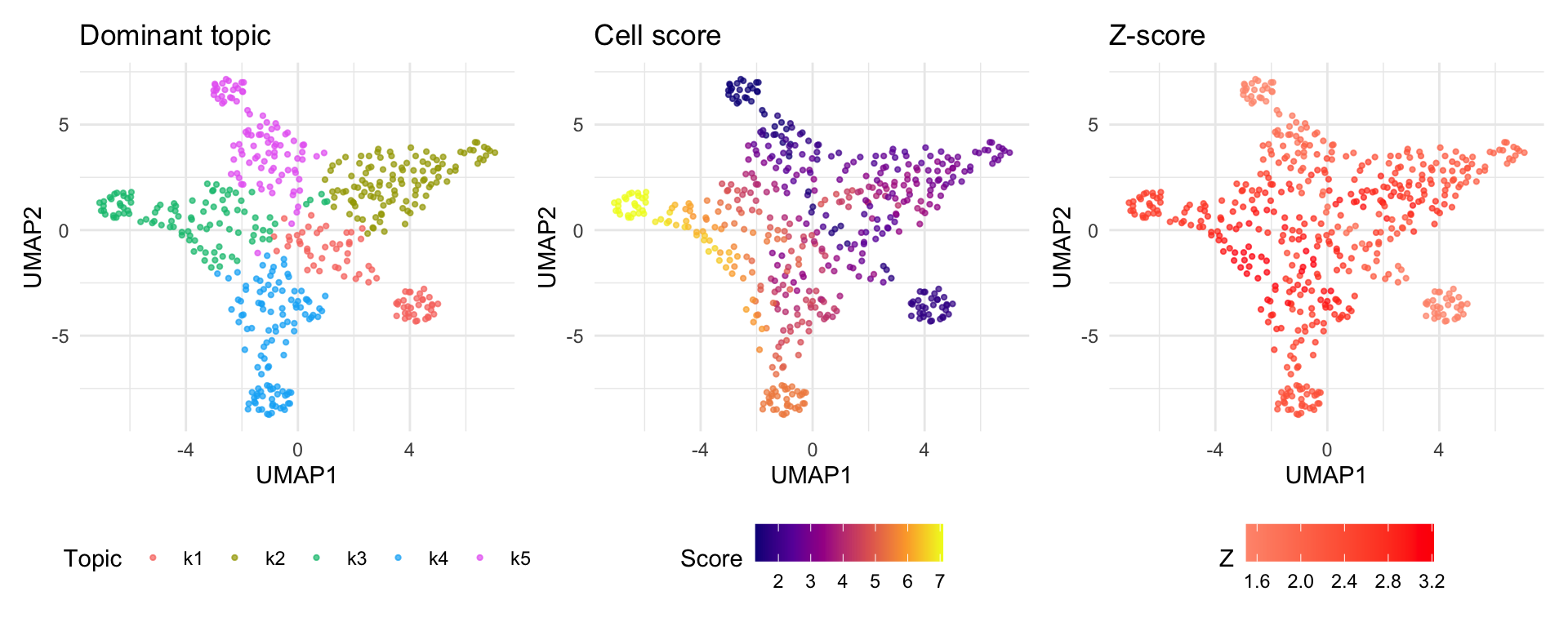
Cells dominated by topics with high enrichment (e.g., k3, k4) show elevated scores, while cells in low-enrichment topics score near the baseline.
Next steps
- See the Step-by-Step Tutorial for a detailed walkthrough of each pipeline stage, diagnostic plots, and parameter explanations.
- For a real analysis, use
chrs = 1:22to run on all chromosomes. - Use
resume_from_stepto re-run specific steps without starting over.