scads: Step-by-Step Tutorial

Overview

scads (Single-Cell ATAC-seq Disease Scoring) computes per-cell disease relevance scores by combining single-cell chromatin accessibility data with GWAS summary statistics. The pipeline has four main steps:

Step	What it does	Typical runtime	Peak memory
1. fastTopics	Fits a topic model on the count matrix, identifies topic-specific peaks via differential expression, and computes a GC-content baseline correction.	~1 min (500 cells, 13K peaks, 5 topics)	~650 MB
2. Topic annotations	Converts significant peaks per topic into BED files for S-LDSC.	< 10 sec	Negligible
3. S-LDSC	Runs stratified LD score regression for each topic using the baseline LD v2.2 model. This is the most time-consuming step.	~10 min per topic per chromosome (sequential)	~300 MB per topic (Python)
4. Cell scores	Combines S-LDSC enrichment estimates with cell-level topic loadings to produce a per-cell disease score.	< 10 sec	~650 MB

Note on runtime: The times above were measured on a MacBook Pro (M3 Max, 36 GB RAM) using the demo dataset (500 cells, 12,971 peaks on chr10, 5 topics). A full-genome analysis (22 chromosomes) will take proportionally longer for Step 3. Larger datasets (more cells or peaks) will increase Step 1 runtime.

Prerequisites

Before running this tutorial, make sure you have completed all installation steps described in the README:

polyFUN and LDSC are cloned and the polyfun conda environment is set up (Python 3.11, with bitarray<3 and bedtools installed).
scads R package is installed with all dependencies.
S-LDSC reference data has been downloaded (see below).

Download S-LDSC reference data

scads requires reference files from the S-LDSC baseline LD model. Download and extract them into a local directory (e.g., ~/LDSCORE/). All files are available from Zenodo.

Disk usage: The compressed downloads total ~1 GB. After extraction, the reference data requires ~4 GB of disk space.

# Create a directory for the reference data
mkdir -p ~/LDSCORE

# Download reference files from Zenodo (~1 GB total)
cd ~/LDSCORE
curl -fSL -o 1000G_Phase3_plinkfiles.tgz \
  "https://zenodo.org/records/10515792/files/1000G_Phase3_plinkfiles.tgz?download=1"            # 275 MB
curl -fSL -o 1000G_Phase3_baselineLD_v2.2_ldscores.tgz \
  "https://zenodo.org/records/10515792/files/1000G_Phase3_baselineLD_v2.2_ldscores.tgz?download=1"  # 645 MB
curl -fSL -o 1000G_Phase3_frq.tgz \
  "https://zenodo.org/records/10515792/files/1000G_Phase3_frq.tgz?download=1"                   # 82 MB
curl -fSL -o 1000G_Phase3_weights_hm3_no_MHC.tgz \
  "https://zenodo.org/records/10515792/files/1000G_Phase3_weights_hm3_no_MHC.tgz?download=1"    # 12 MB
curl -fSL -o hm3_no_MHC.list.txt \
  "https://zenodo.org/records/10515792/files/hm3_no_MHC.list.txt?download=1"                    # 12 MB

# Extract archives
tar -xzf 1000G_Phase3_plinkfiles.tgz
tar -xzf 1000G_Phase3_frq.tgz
tar -xzf 1000G_Phase3_weights_hm3_no_MHC.tgz

# The baseline LD archive extracts files directly (not into a subdirectory),
# so create one first:
mkdir -p 1000G_Phase3_baselineLD_v2.2_ldscores
tar -xzf 1000G_Phase3_baselineLD_v2.2_ldscores.tgz -C 1000G_Phase3_baselineLD_v2.2_ldscores

# (Optional) Remove the .tgz files to free ~1 GB of disk space
# rm -f *.tgz

After extraction, you should have the following directory structure:

~/LDSCORE/
├── 1000G_EUR_Phase3_plink/          # 1000G.EUR.QC.{1..22}.{bed,bim,fam}
├── 1000G_Phase3_baselineLD_v2.2_ldscores/  # baselineLD.{1..22}.{annot.gz,l2.ldscore.gz,...}
├── 1000G_Phase3_frq/                # 1000G.EUR.QC.{1..22}.frq
├── 1000G_Phase3_weights_hm3_no_MHC/ # weights.hm3_noMHC.{1..22}.l2.ldscore.gz
└── hm3_no_MHC.list.txt

Start an R session

Activate the polyfun conda environment before starting R. This ensures that python3 (called internally by scads) resolves to the environment with the required Python packages (including ldsc, polyfun, bedtools, bitarray<3).

conda activate polyfun
R

Load the scads package:

library(scads)
library(data.table)
library(ggplot2)

Load example data

scads ships with a small demo dataset:

demo_count_matrix: A sparse peak-by-cell count matrix (12,971 peaks on chr10 x 500 cells) from scATAC-seq data.
SIM_sumstats_chr10.txt.gz: Simulated GWAS summary statistics for chromosome 10.

# Load demo peak-by-cell count matrix
data("demo_count_matrix")

# Examine the dataset
cat("Dimensions (peaks x cells):", dim(demo_count_matrix), "\n")
#> Dimensions (peaks x cells): 12971 500
cat("Matrix class:", class(demo_count_matrix), "\n")
#> Matrix class: dgCMatrix
cat("Non-zero entries:", length(demo_count_matrix@x), "\n")
#> Non-zero entries: 521704
cat("Sparsity:", round(1 - length(demo_count_matrix@x) / prod(dim(demo_count_matrix)), 4), "\n")
#> Sparsity: 0.9196
demo_count_matrix[1:5, 1:5]
#> 5 x 5 sparse Matrix of class "dgCMatrix"
#>                                    
#> chr10:8380739-8381239     . . . . .
#> chr10:131742591-131743091 . . . . 1
#> chr10:74486605-74487105   . . 1 . .
#> chr10:42737563-42738063   . . . . .
#> chr10:88092916-88093416   . . . . .

The count matrix is a sparse matrix where rows are genomic peaks (in chr:start-end format) and columns are cells. Most entries are zero, which is typical for scATAC-seq data.

Load the example GWAS summary statistics:

data_file <- system.file("extdata", "SIM_sumstats_chr10.txt.gz", package = "scads")
sumstats <- fread(data_file, header = TRUE)
cat("Summary statistics dimensions:", dim(sumstats), "\n")
#> Summary statistics dimensions: 292171 9
cat("Columns:", paste(names(sumstats), collapse = ", "), "\n")
#> Columns: chr, pos, beta, se, a0, a1, snp, pval, zscore
head(sumstats)
#>      chr   pos        beta         se     a0     a1         snp      pval
#>    <int> <int>       <num>      <num> <char> <char>      <char>     <num>
#> 1:    10 88766  0.05890450 0.02166930      T      C  rs55896525 0.0065637
#> 2:    10 90127  0.00707272 0.01724490      T      C rs185642176 0.6817090
#> 3:    10 90164  0.00943048 0.01800330      G      C rs141504207 0.6004070
#> 4:    10 94426 -0.00194658 0.00975979      T      C  rs10904045 0.8419120
#> 5:    10 95074 -0.00011268 0.00960219      A      G   rs6560828 0.9906370
#> 6:    10 95662 -0.01198410 0.01025610      C      G  rs35849539 0.2426170
#>         zscore
#>          <num>
#> 1:  2.71833885
#> 2:  0.41013401
#> 3:  0.52381952
#> 4: -0.19944896
#> 5: -0.01173482
#> 6: -1.16848510

The summary statistics file must contain columns: chr, pos, beta, se, a0 (ref allele), a1 (alt allele), snp (rsID), pval, and zscore.

Configure paths

Set the paths to match your local environment. You need to specify:

polyfun_d / ldsc_d: where polyFUN and LDSC are cloned.
ldscore_dir: where the S-LDSC reference data was downloaded.
output_dir: where scads will write its results.

# -- User-specific paths (edit these) -----------------------------------------
polyfun_d    <- path.expand("~/polyfun/")
ldsc_d       <- path.expand("~/ldsc/")
ldscore_dir  <- path.expand("~/Desktop/Project_scads/LDSCORE/zenodo/")
output_dir   <- path.expand("~/scads_output/")

# -- Reference data paths (derived from ldscore_dir) --------------------------
onekg_pref    <- file.path(ldscore_dir, "1000G_EUR_Phase3_plink", "1000G.EUR.QC.")
baseline_pref <- file.path(ldscore_dir, "1000G_Phase3_baselineLD_v2.2_ldscores", "baselineLD.")
frq_pref      <- file.path(ldscore_dir, "1000G_Phase3_frq", "1000G.EUR.QC.")
hm3_file      <- file.path(ldscore_dir, "hm3_no_MHC.list.txt")
weights_pref  <- file.path(ldscore_dir, "1000G_Phase3_weights_hm3_no_MHC", "weights.hm3_noMHC.")

Verify that the key files exist before proceeding:

dir.create(output_dir, showWarnings = FALSE, recursive = TRUE)
stopifnot(
  "polyfun ldsc.py not found"    = file.exists(file.path(polyfun_d, "ldsc.py")),
  "ldsc make_annot.py not found" = file.exists(file.path(ldsc_d, "make_annot.py")),
  "1000G plink files not found"  = file.exists(paste0(onekg_pref, "10.bim")),
  "Baseline LD files not found"  = file.exists(paste0(baseline_pref, "10.l2.ldscore.gz")),
  "Frequency files not found"    = file.exists(paste0(frq_pref, "10.frq")),
  "HapMap3 SNP list not found"   = file.exists(hm3_file),
  "Weight files not found"       = file.exists(paste0(weights_pref, "10.l2.ldscore.gz"))
)
cat("All paths verified.\n")
#> All paths verified.

Set analysis parameters

count_matrix <- demo_count_matrix
n_topics     <- 5       # number of topics to fit
n_sims       <- 1000    # Monte Carlo samples for DE analysis
n_cores      <- 8       # adjust to the number of cores available
bl_method    <- "gc"    # GC-content baseline correction (recommended)
bl_ct        <- NULL    # cell type for "estimate" baseline (not used here)
bl_peaks     <- NULL    # cell type peaks for "estimate" baseline (not used here)
sumstats_d   <- dirname(data_file)
gwas_n       <- 45087   # GWAS sample size
trait         <- "SIM"
cont_topics  <- FALSE   # use binary (not continuous) topic annotations

Baseline method options

The baseline_method parameter controls how the null hypothesis is set for differential expression testing in Step 1:

Method	Description
`"gc"`	(Recommended) Fits a GC-content-dependent baseline using an EM algorithm with a Poisson mixture model. Accounts for GC bias in chromatin accessibility.
`"constant"`	Uses a fixed small constant (`1e-7`) as baseline. Simple but does not account for GC bias.
`"average"`	Computes a genome-wide average accessibility rate.
`"estimate"`	Estimates background from a reference cell type’s non-overlapping peaks. Requires `bl_celltype` and `bl_celltype_peak_file`.

Running the pipeline step by step

While scads() can run the entire pipeline in one call, this tutorial walks through each step individually to show intermediate results. The scads() wrapper calls these same functions internally and supports checkpointing via save_intermediates = TRUE and resume_from_step.

Note: This tutorial runs on chromosome 10 only (chrs = 10) to keep runtime short (~50 min total). For a real analysis, use chrs = 1:22.

Step 1: Fit topic model with fastTopics

What this step does:

Transposes the count matrix (peaks x cells -> cells x peaks) for fastTopics.
Fits a Poisson NMF topic model with k topics using fastTopics::fit_topic_model().
Computes a GC-content baseline correction for each topic (if baseline_method = "gc").
Runs differential expression analysis to identify topic-specific peaks.
Applies FDR correction and binarizes peak assignments.

Runtime: ~1 min for the demo dataset (500 cells, 12,971 peaks, 5 topics). Memory: ~650 MB peak.

out1_cache <- file.path(output_dir, "run_fastTopics_res.rds")
if (file.exists(out1_cache)) {
  cat("Loading cached Step 1 results from", out1_cache, "\n")
  out1 <- readRDS(out1_cache)
} else {
  set.seed(1234)

  # Transpose: scads expects peaks-by-cells, but fastTopics needs cells-by-peaks
  count_matrix_t <- Matrix::t(count_matrix)
  cat("Input dimensions (cells x peaks):", dim(count_matrix_t), "\n")

  # Run fastTopics
  t1_start <- Sys.time()
  out1 <- run_fastTopics(
    count_matrix  = count_matrix_t,
    nTopics       = n_topics,
    n_s           = n_sims,
    n_c           = n_cores,
    baseline_method = bl_method,
    bl_celltype_cells = bl_ct,
    bl_celltype_peak_file = bl_peaks,
    fdr_cutoff    = 0.05,
    outdir        = output_dir,
    genome        = "hg19"
  )
  t1_end <- Sys.time()
  cat("\nStep 1 runtime:", round(difftime(t1_end, t1_start, units = "secs")), "seconds\n")

  # Save intermediate results
  saveRDS(out1, out1_cache)
}
#> Loading cached Step 1 results from /Users/siming/scads_output//run_fastTopics_res.rds

Examine Step 1 results:

# Topic model dimensions
cat("Factor matrix F (peaks x topics):", dim(out1$Fmat), "\n")
#> Factor matrix F (peaks x topics): 12971 5
cat("Loading matrix L (cells x topics):", dim(out1$Lmat), "\n")
#> Loading matrix L (cells x topics): 500 5
cat("Binary peak matrix P (peaks x topics):", dim(out1$Pmat), "\n")
#> Binary peak matrix P (peaks x topics): 12971 5

# Number of significant peaks per topic (after FDR correction)
cat("\nSignificant peaks per topic:\n")
#> 
#> Significant peaks per topic:
print(colSums(out1$Pmat))
#>   k1   k2   k3   k4   k5 
#> 3995 8380 6827 5417 6309

The binary peak matrix Pmat indicates which peaks are significantly enriched in each topic (1 = significant at FDR < 0.05). These will be used as topic annotations for S-LDSC.

Step 2: Generate topic annotation BED files

What this step does:

Converts the binary peak-topic assignments (Pmat) into BED files for each topic. Each BED file contains the genomic coordinates of peaks assigned to that topic, which S-LDSC uses as a custom annotation.

Runtime: < 10 seconds. Memory: Negligible.

beddir_cache <- file.path(output_dir, "beddir_list.rds")
if (file.exists(beddir_cache)) {
  cat("Loading cached Step 2 results from", beddir_cache, "\n")
  beddir_list <- readRDS(beddir_cache)
} else {
  t2_start <- Sys.time()
  beddir_list <- get_annot_beds(topics_res = out1, output_dir = output_dir)
  t2_end <- Sys.time()
  cat("Step 2 runtime:", round(difftime(t2_end, t2_start, units = "secs"), 1), "seconds\n")

  # Save for checkpointing
  saveRDS(beddir_list, beddir_cache)
}
#> Loading cached Step 2 results from /Users/siming/scads_output//beddir_list.rds

Step 3: Run S-LDSC per topic

What this step does:

For each topic annotation, this step runs the full S-LDSC pipeline:

Munge summary statistics – converts GWAS sumstats to the format expected by LDSC (parquet file via munge_polyfun_sumstats.py).
Create annotation – for each chromosome, marks which 1000G SNPs fall within topic peaks (via make_annot.py).
Compute LD scores – calculates LD scores for the custom annotation (via ldsc.py --l2).
Heritability estimation – runs partitioned heritability analysis combining the custom annotation with the baseline LD v2.2 model (via ldsc.py --h2).

The key output is the enrichment estimate per topic: how much heritability is concentrated in the topic’s peaks relative to their size.

Runtime: ~10 min per topic per chromosome. With 5 topics on chr10 running sequentially, expect ~50 min total. Memory: ~300 MB per topic (Python processes).

# Check which topics already have S-LDSC results
t3_start <- Sys.time()
all_done <- all(vapply(seq_along(beddir_list), function(i) {
  file.exists(file.path(beddir_list[[i]], "results", paste0(trait, ".results")))
}, logical(1)))

if (all_done) {
  cat("All S-LDSC results found — skipping Step 3.\n")
} else {
  for (i in seq_along(beddir_list)) {
    res_file <- file.path(beddir_list[[i]], "results", paste0(trait, ".results"))
    if (file.exists(res_file)) {
      cat(sprintf("--- Topic %d already done, skipping ---\n", i))
      next
    }
    cat(sprintf("\n--- Running S-LDSC for topic %d of %d ---\n", i, length(beddir_list)))

    run_sldsc(
      chrs          = 10,                    # chr10 only for this tutorial
      polyfun_path  = polyfun_d,
      ldsc_path     = ldsc_d,
      sumstats_path = sumstats_d,
      n             = gwas_n,
      trait         = trait,
      onekg_path    = onekg_pref,
      bed_dir       = beddir_list[[i]],
      baseline_dir  = baseline_pref,
      frqfile_pref  = frq_pref,
      hm3_snps      = hm3_file,
      weights_pref  = weights_pref,
      out_dir       = beddir_list[[i]]
    )
  }
}
#> All S-LDSC results found — skipping Step 3.
t3_end <- Sys.time()
cat("\nStep 3 total runtime:", round(difftime(t3_end, t3_start, units = "secs"), 1), "seconds\n")
#> 
#> Step 3 total runtime: 0 seconds

The enrichment results per topic are displayed after Step 4 (which reads and processes the S-LDSC output files).

Step 4: Calculate cell scores

What this step does:

Combines the S-LDSC enrichment estimates with cell-level topic loadings to produce a per-cell disease relevance score:

Reads S-LDSC results for each topic and applies adaptive shrinkage (ASH) to stabilize enrichment estimates.
Computes a weighted score per cell: cs_i = sum(L_ik * a_k * e_k) / sum(L_ik * a_k), where L_ik is the cell’s loading on topic k, a_k is the number of peaks in topic k, and e_k is the (shrunk) enrichment estimate.
Computes z-scores and p-values accounting for correlation between topic annotations.

Runtime: < 10 seconds. Memory: ~650 MB (due to correlation matrix computation).

cs_cache <- file.path(output_dir, "cs_res.rds")
if (file.exists(cs_cache)) {
  cat("Loading cached Step 4 results from", cs_cache, "\n")
  cs_res <- readRDS(cs_cache)
} else {
  t4_start <- Sys.time()
  cs_res <- get_cs(
    topic_res    = out1,
    ldsc_res_dir = output_dir,
    trait        = trait,
    nTopics      = n_topics
  )
  t4_end <- Sys.time()
  cat("Step 4 runtime:", round(difftime(t4_end, t4_start, units = "secs"), 1), "seconds\n")

  # Save results
  saveRDS(cs_res, cs_cache)
}
#> Loading cached Step 4 results from /Users/siming/scads_output//cs_res.rds

Examine Step 4 results:

cat("Cell score summary:\n")
#> Cell score summary:
print(summary(cs_res$cs))
#>    Min. 1st Qu.  Median    Mean 3rd Qu.    Max. 
#>   1.291   2.472   3.544   3.780   5.172   7.089

cat("\nZ-score summary:\n")
#> 
#> Z-score summary:
print(summary(as.numeric(cs_res$z_cell)))
#>    Min. 1st Qu.  Median    Mean 3rd Qu.    Max. 
#>   1.500   2.155   2.503   2.401   2.738   3.216

cat("\nNumber of significant cells (p < 0.05):", sum(cs_res$p_cell < 0.05), "\n")
#> 
#> Number of significant cells (p < 0.05): 413
cat("Number of significant cells (p < 0.01):", sum(cs_res$p_cell < 0.01), "\n")
#> Number of significant cells (p < 0.01): 220

cat("\nASH-shrunk enrichment estimates:\n")
#> 
#> ASH-shrunk enrichment estimates:
print(cs_res$ash_res$PosteriorMean)
#> [1] 1.804256 2.697942 7.089065 5.443484 1.291199

Understanding the output:

cs: The per-cell disease score. Higher values indicate greater disease relevance based on the cell’s chromatin accessibility profile.
z_cell: Z-score for each cell, accounting for variance in enrichment estimates and correlation between topic annotations.
p_cell: Two-sided p-value for each cell’s score.
ldsc_res_table: Raw S-LDSC results per topic.
ash_res: Enrichment estimates after adaptive shrinkage (more stable).
cs_dat: Intermediate values (M_i, N_i) used in score computation.

Higher cell scores indicate cells whose chromatin accessibility profiles overlap more strongly with disease-associated regions. Cells dominated by topics with high enrichment will receive higher scores.

Visualizing results

After running the pipeline, it is important to inspect intermediate and final results. This section shows diagnostic plots for each stage.

Topic model diagnostics

Distribution of factor loadings (Fmat)

The factor loading matrix Fmat (peaks x topics) contains the Poisson rate parameters for each peak in each topic. Examining the distribution of log10(F) per topic reveals whether the model separates foreground (high F) from background (low F) peaks.

Fmat <- out1$Fmat

# Histogram of log10(Fmat) per topic
fmat_df <- do.call(rbind, lapply(1:ncol(Fmat), function(k) {
  data.frame(
    log10F = log10(Fmat[, k]),
    topic  = paste0("k", k)
  )
}))

ggplot(fmat_df, aes(x = log10F)) +
  geom_histogram(bins = 100, fill = "steelblue", color = "white", linewidth = 0.1) +
  facet_wrap(~topic, scales = "free_y") +
  labs(title = "Distribution of log10(F) per topic",
       x = "log10(F)", y = "Count") +
  theme_minimal()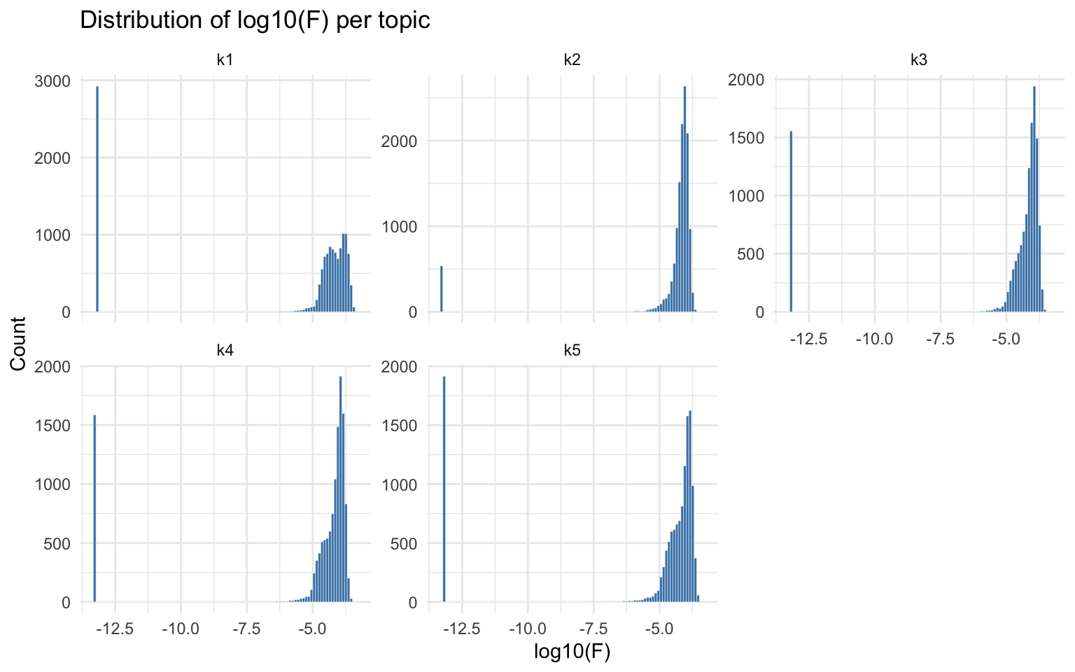

Structure plot

The fastTopics structure plot shows how cells are distributed across topics. Each vertical bar represents a cell, colored by its topic proportions (from the Lmat loading matrix). Cells dominated by a single topic form clusters.

fastTopics::structure_plot(out1$fastTopics_fit)
#> Running tsne on 500 x 5 matrix.
#> Read the 500 x 5 data matrix successfully!
#> Using no_dims = 1, perplexity = 100.000000, and theta = 0.100000
#> Computing input similarities...
#> Building tree...
#> Done in 0.08 seconds (sparsity = 0.769136)!
#> Learning embedding...
#> Iteration 50: error is 48.722003 (50 iterations in 0.04 seconds)
#> Iteration 100: error is 48.722003 (50 iterations in 0.04 seconds)
#> Iteration 150: error is 48.722003 (50 iterations in 0.04 seconds)
#> Iteration 200: error is 48.722003 (50 iterations in 0.04 seconds)
#> Iteration 250: error is 48.722003 (50 iterations in 0.04 seconds)
#> Iteration 300: error is 0.446991 (50 iterations in 0.04 seconds)
#> Iteration 350: error is 0.440582 (50 iterations in 0.03 seconds)
#> Iteration 400: error is 0.440534 (50 iterations in 0.04 seconds)
#> Iteration 450: error is 0.440535 (50 iterations in 0.03 seconds)
#> Iteration 500: error is 0.440536 (50 iterations in 0.03 seconds)
#> Iteration 550: error is 0.440536 (50 iterations in 0.03 seconds)
#> Iteration 600: error is 0.440536 (50 iterations in 0.04 seconds)
#> Iteration 650: error is 0.440536 (50 iterations in 0.04 seconds)
#> Iteration 700: error is 0.440536 (50 iterations in 0.03 seconds)
#> Iteration 750: error is 0.440536 (50 iterations in 0.03 seconds)
#> Iteration 800: error is 0.440536 (50 iterations in 0.04 seconds)
#> Iteration 850: error is 0.440536 (50 iterations in 0.04 seconds)
#> Iteration 900: error is 0.440536 (50 iterations in 0.04 seconds)
#> Iteration 950: error is 0.440536 (50 iterations in 0.04 seconds)
#> Iteration 1000: error is 0.440536 (50 iterations in 0.03 seconds)
#> Fitting performed in 0.72 seconds.
#> Warning: `aes_string()` was deprecated in ggplot2 3.0.0.
#> ℹ Please use tidy evaluation idioms with `aes()`.
#> ℹ See also `vignette("ggplot2-in-packages")` for more information.
#> ℹ The deprecated feature was likely used in the fastTopics package.
#>   Please report the issue at
#>   <https://github.com/stephenslab/fastTopics/issues>.
#> This warning is displayed once per session.
#> Call `lifecycle::last_lifecycle_warnings()` to see where this warning was
#> generated.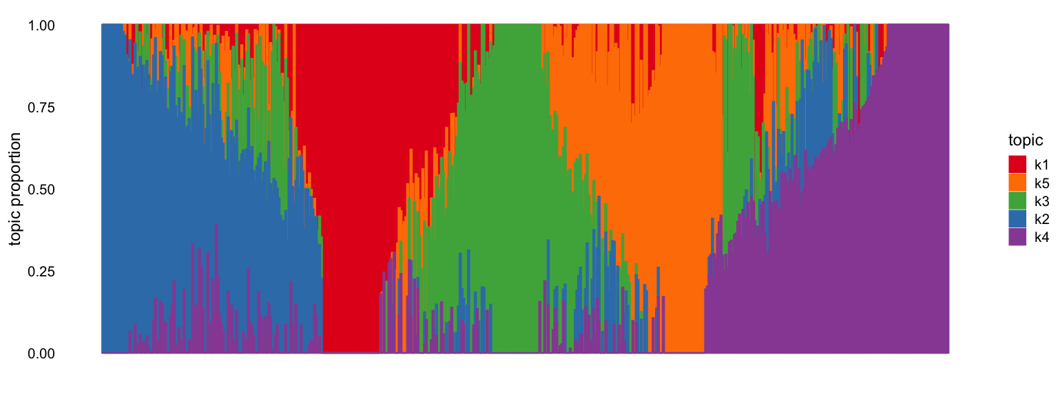

S-LDSC enrichment summary

Enrichment bar plot

Visualizing enrichment estimates with error bars helps identify which topics carry disease signal. Topics with positive enrichment (and small standard error) are the informative ones.

ldsc_tab <- cs_res$ldsc_res_table

# Add ASH-shrunk estimates
ldsc_tab$ASH_Enrichment <- cs_res$ash_res$PosteriorMean

# Bar plot of enrichment per topic
ggplot(ldsc_tab, aes(x = Category, y = Enrichment)) +
  geom_col(fill = "steelblue", width = 0.6) +
  geom_errorbar(aes(ymin = Enrichment - 1.96 * Enrichment_std_error,
                     ymax = Enrichment + 1.96 * Enrichment_std_error),
                width = 0.2) +
  geom_hline(yintercept = 1, linetype = "dashed", color = "red") +
  labs(title = "S-LDSC enrichment per topic",
       subtitle = "Dashed line = no enrichment (1.0). Error bars = 95% CI.",
       x = "Topic", y = "Enrichment") +
  theme_minimal()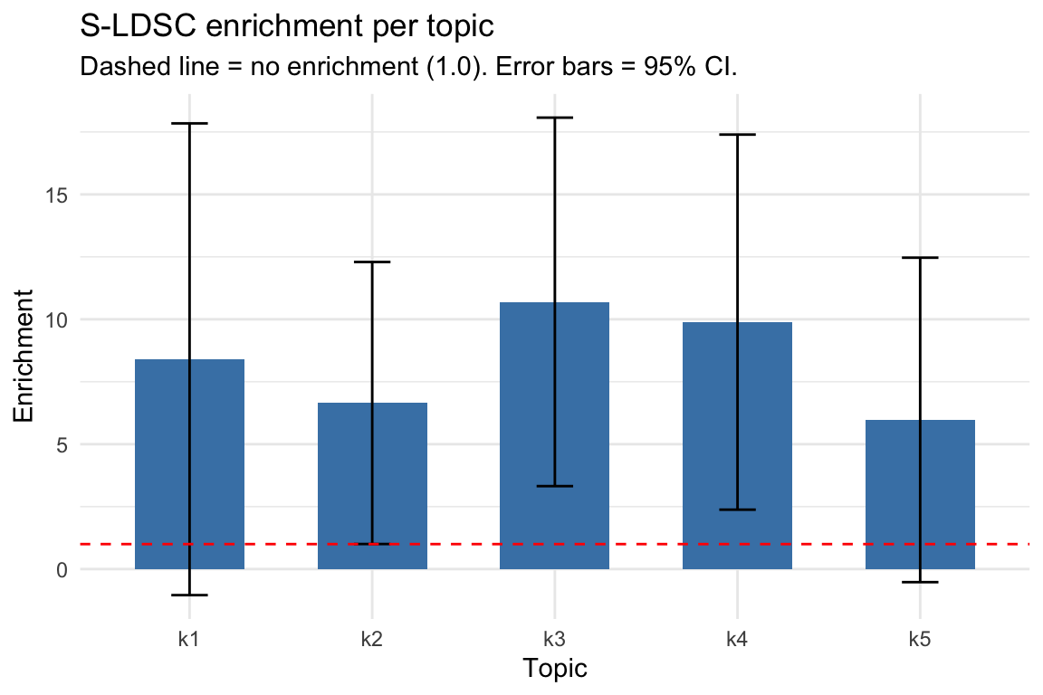

S-LDSC results table

# Full results table
print(ldsc_tab[, c("Category", "Prop._SNPs", "Prop._h2", "Enrichment",
                    "Enrichment_std_error", "ASH_Enrichment")])
#>   Category Prop._SNPs Prop._h2 Enrichment Enrichment_std_error ASH_Enrichment
#> 1       k1   0.014473  0.12158     8.4002               4.8179       1.804256
#> 2       k2   0.030417  0.20225     6.6492               2.8804       2.697942
#> 3       k3   0.024685  0.26406    10.6970               3.7634       7.089065
#> 4       k4   0.019800  0.19575     9.8865               3.8306       5.443484
#> 5       k5   0.022393  0.13373     5.9718               3.3137       1.291199

Interpreting enrichment: Enrichment > 1 means heritability is concentrated in a topic’s peaks more than expected by chance. Topics with enrichment significantly > 1 (confidence interval not crossing 1) indicate disease-relevant chromatin programs. After adaptive shrinkage (ASH), the estimates are stabilized and used to weight cell scores in Step 4.

Cell score distribution

Histogram of cell scores

cs_df <- data.frame(cs = cs_res$cs)

ggplot(cs_df, aes(x = cs)) +
  geom_histogram(bins = 50, fill = "steelblue", color = "white") +
  labs(title = "Distribution of cell scores",
       x = "Cell score", y = "Count") +
  theme_minimal()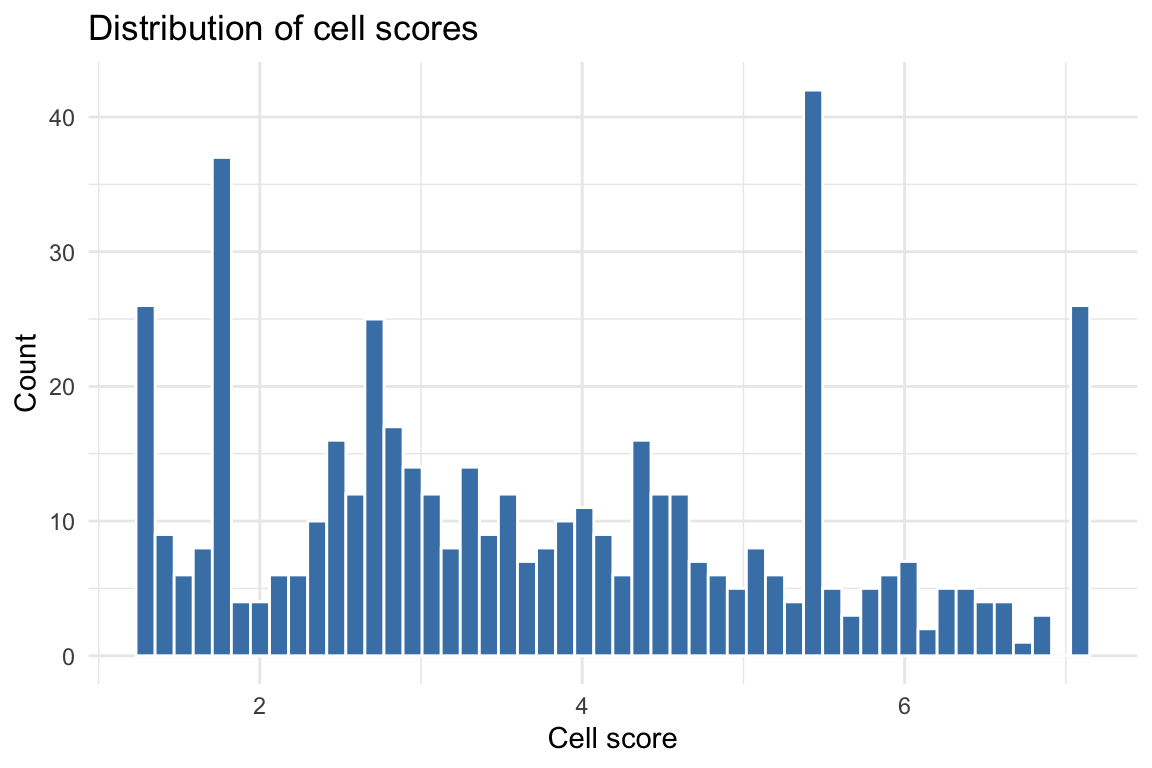

Z-score distribution

The z-scores account for variance in enrichment estimates and correlation between topic annotations. Under the null (no disease signal), z-scores should be approximately standard normal.

z_df <- data.frame(z = as.numeric(cs_res$z_cell))
z_df <- z_df[is.finite(z_df$z), , drop = FALSE]

ggplot(z_df, aes(x = z)) +
  geom_histogram(bins = 50, fill = "steelblue", color = "white") +
  geom_vline(xintercept = c(-1.96, 1.96), linetype = "dashed", color = "red") +
  labs(title = "Distribution of cell z-scores",
       subtitle = "Dashed lines = +/-1.96 (p = 0.05 threshold)",
       x = "Z-score", y = "Count") +
  theme_minimal()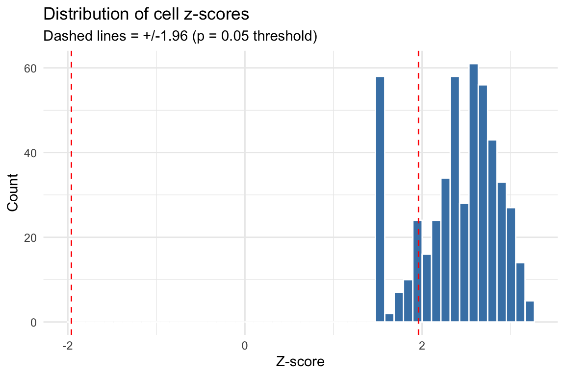

UMAP visualization

UMAP provides a 2D embedding of cells based on the topic loading matrix (Lmat). Coloring cells by their disease score reveals whether disease-relevant cells cluster together.

if (!requireNamespace("uwot", quietly = TRUE)) {
  message("Install 'uwot' for UMAP: install.packages('uwot')")
} else {
  library(patchwork)

  # Compute UMAP from topic loadings
  set.seed(42)
  umap_coords <- uwot::umap(out1$Lmat, n_neighbors = 350, min_dist = 0.8)

  umap_df <- data.frame(
    UMAP1 = umap_coords[, 1],
    UMAP2 = umap_coords[, 2],
    cell_score = cs_res$cs,
    z_score = as.numeric(cs_res$z_cell)
  )

  # Color by dominant topic
  dominant_topic <- paste0("k", apply(out1$Lmat, 1, which.max))
  umap_df$topic <- dominant_topic

  p3 <- ggplot(umap_df, aes(x = UMAP1, y = UMAP2, color = topic)) +
    geom_point(size = 0.8, alpha = 0.7) +
    labs(title = "Dominant topic", color = "Topic") +
    theme_minimal() + theme(legend.position = "bottom")

  # Color by cell score
  p1 <- ggplot(umap_df, aes(x = UMAP1, y = UMAP2, color = cell_score)) +
    geom_point(size = 0.8, alpha = 0.7) +
    scale_color_viridis_c(option = "C") +
    labs(title = "Cell score", color = "Score") +
    theme_minimal() + theme(legend.position = "bottom")

  # Color by z-score
  p2 <- ggplot(umap_df, aes(x = UMAP1, y = UMAP2, color = z_score)) +
    geom_point(size = 0.8, alpha = 0.7) +
    scale_color_gradient2(low = "blue", mid = "grey90", high = "red", midpoint = 0) +
    labs(title = "Z-score", color = "Z") +
    theme_minimal() + theme(legend.position = "bottom")

  # Combine plots
  p3 + p1 + p2 + plot_layout(ncol = 3)
}

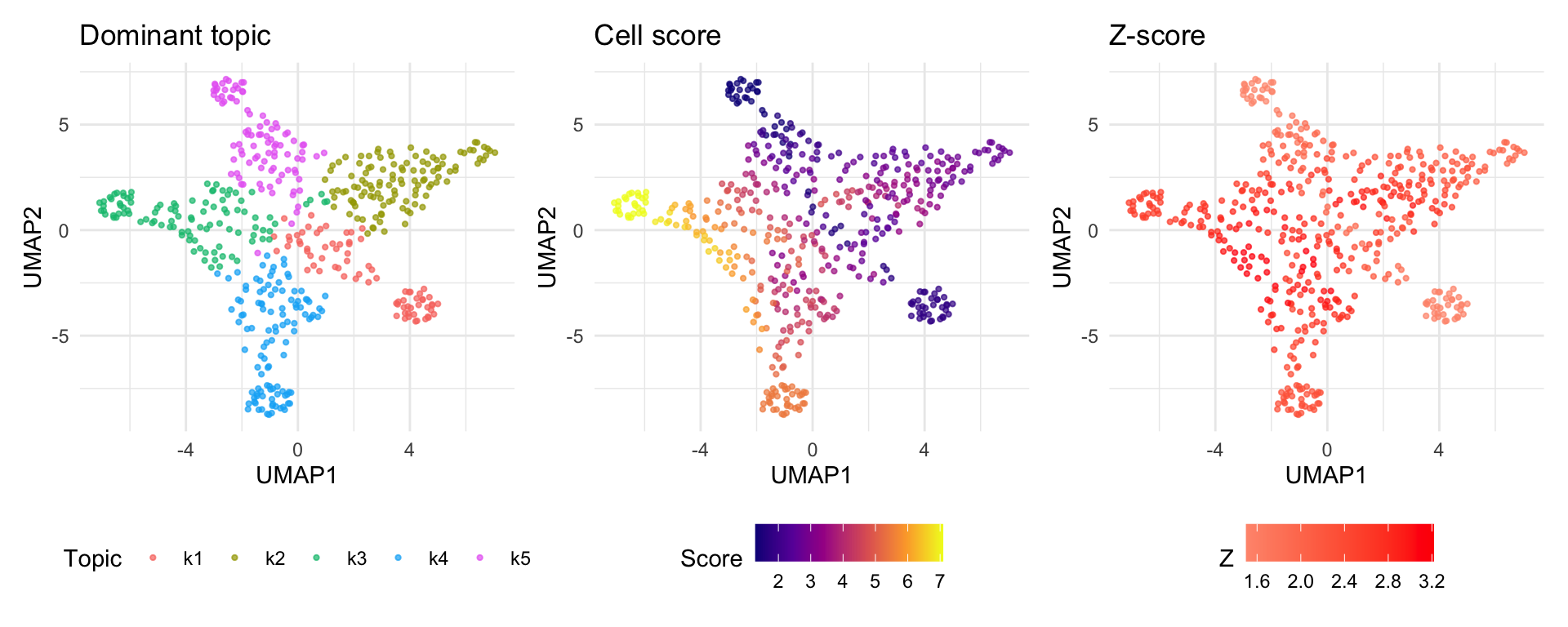
Note: Cells dominated by topics with high enrichment will appear as “hot spots” on the score UMAP. The z-score UMAP highlights cells whose scores are statistically significant after accounting for estimation uncertainty and topic correlation.

Running the full pipeline with `scads()`

Instead of running each step manually, you can use scads() to run the entire pipeline in one call. The updated scads() function supports:

save_intermediates = TRUE (default): Saves intermediate RDS files at each step for inspection and checkpointing.
resume_from_step: Resume from step 1, 2, 3, or 4, loading prior results from outdir.
verbose = TRUE (default): Prints time stamped progress messages.

set.seed(1234)
scads_res <- scads(
  count_matrix,
  nTopics                = n_topics,
  n_s                    = n_sims,
  n_c                    = n_cores,
  baseline_method        = bl_method,
  bl_celltype            = bl_ct,
  bl_celltype_peak_file  = bl_peaks,
  sumstats_dir           = sumstats_d,
  gwas_nsamps            = gwas_n,
  gwas_trait             = trait,
  outdir                 = output_dir,
  polyfun_code_dir       = polyfun_d,
  ldsc_code_dir          = ldsc_d,
  onekg_path             = onekg_pref,
  baseline_dir           = baseline_pref,
  frqfile_pref           = frq_pref,
  hm3_snps               = hm3_file,
  weights_pref           = weights_pref,
  continuous_topic_annot = cont_topics,
  chrs                   = 10,
  genome                 = "hg19",
  save_intermediates     = TRUE,
  verbose                = TRUE
)

Resuming from a checkpoint

If Step 3 (S-LDSC) completed but you want to re-run Step 4 with different parameters, or if the pipeline was interrupted, you can resume:

# Resume from Step 4 (loads fastTopics results and BED dirs from saved files)
scads_res <- scads(
  count_matrix,
  nTopics         = n_topics,
  sumstats_dir    = sumstats_d,
  gwas_nsamps     = gwas_n,
  gwas_trait      = trait,
  outdir          = output_dir,
  polyfun_code_dir = polyfun_d,
  ldsc_code_dir   = ldsc_d,
  onekg_path      = onekg_pref,
  baseline_dir    = baseline_pref,
  frqfile_pref    = frq_pref,
  hm3_snps        = hm3_file,
  weights_pref    = weights_pref,
  chrs            = 10,
  resume_from_step = 4
)

Output files

After running the pipeline, output_dir contains:

output_dir/
├── run_fastTopics_res.rds          # Step 1 results (fastTopics model + DE)
├── fasTopics_fit.rds               # Raw fastTopics model fit
├── count_mat_tp.rds                # Pseudobulk count matrix (peaks x topics)
├── beddir_list.rds                 # Step 2 results (BED directory paths)
├── cs_res.rds                      # Step 4 results (cell scores)
├── k1_output/                      # Topic 1
│   ├── k1_annotations.bed          #   BED file of topic peaks
│   ├── annotations/SIM/            #   S-LDSC annotation files
│   │   └── SIM.10.{annot.gz,l2.ldscore.gz,...}
│   ├── results/                    #   S-LDSC results
│   │   └── SIM.{results,log}
│   └── SIM_munged_sumstats.parquet #   Munged GWAS sumstats
├── k2_output/                      # Topic 2 (same structure)
│   └── ...
└── k5_output/                      # Topic 5
    └── ...

The result list returned by scads() has two elements:

out1: The fitted fastTopics model, including:
- fastTopics_fit: The raw topic model object
- Fmat: Factor loadings matrix (peaks x topics)
- Lmat: Topic proportions matrix (cells x topics)
- Pmat: Binary peak assignments (peaks x topics)
- de_res: Full differential expression results (z-scores, log-fold changes)
- baseline: The GC-content baseline used for DE testing
cs_res: The per-cell disease scores, including:
- cs: Cell score vector
- z_cell: Z-scores per cell
- p_cell: P-values per cell
- ldsc_res_table: S-LDSC results per topic
- ash_res: ASH-stabilized enrichment estimates
- cs_dat: Intermediate M_i and N_i values

Troubleshooting

Common issues

Issue	Solution
`"sortBed" does not appear to be installed`	Install bedtools in your conda env: `conda install -n polyfun -c bioconda bedtools`
`TypeError: float() argument must be a string or a real number, not 'bitarray.decodeiterator'`	Downgrade bitarray: `pip install 'bitarray<3'`
`could not find function "width"`	Make sure `GenomicRanges` is loaded (scads handles this internally)
Paths with spaces break S-LDSC	scads v0.2.0+ handles this via `shQuote()`. If using older versions, use symlinks.
S-LDSC takes too long	Use `chrs = 10` for testing. For production, run on a cluster with `mc.cores`.

2026-03-29

Overview

Prerequisites

Download S-LDSC reference data

Start an R session

Load example data

Configure paths

Set analysis parameters

Baseline method options

Running the pipeline step by step

Step 1: Fit topic model with fastTopics

Step 2: Generate topic annotation BED files

Step 3: Run S-LDSC per topic

Step 4: Calculate cell scores

Visualizing results

Topic model diagnostics

Distribution of factor loadings (Fmat)

Structure plot

S-LDSC enrichment summary

Enrichment bar plot

S-LDSC results table

Cell score distribution

Histogram of cell scores

Z-score distribution

UMAP visualization

Running the full pipeline with scads()

Resuming from a checkpoint

Output files

Troubleshooting

Common issues

Running the full pipeline with `scads()`